
Background
In a randomized or prospectively conducted trial, study entry is identified in a straightforward manner as the formal enrollment of a participant. For example, in a clinical trial evaluating a new drug, study entry could denote the date at which the intervention was initiated, and formal observations and study visits continue after this date. In having a defined time-point, the impact of interventions (comparatively or individually) over time can be evaluated, as it provides a standardized reference for data collection and analysis.
In contrast, consider a set of long-term longitudinal data. Other than the formal enrollment into the study, or the earliest available data point, when can patients be considered “within” a study? Consider a study looking at individuals being treated who are over the age of 50. A patient could be eligible when they are 50, but also when they are 51, 52, and so forth. For scenarios such as this, how can we minimize important sources of temporal bias?
This blog post embarks on a journey through this critical yet often overlooked facet of clinical research. In this post, we’ll share an example where we wish to compare patients treated with local standards of care whose data comes from electronic health records.
Hypothetical Patients
Let us imagine we are interested in comparing patients from a trial (green bar) to patients from an external data source containing long-term data on similar patient populations. Let us assume patients within the randomized trial must have received at least two prior lines of therapy prior to enrollment, and that the endpoint of interest is event-free survival, a time-to-event outcome. Accordingly, assuming all other factors can be mimicked, we require patients from the external population to also have at least two prior lines of therapy. If we focus on hypothetical examples of eligible patients, we identify a challenge from the external data – this patient can have more than one study start date. In contrast, the trial patient has a defined start date, signified by their initiation of the interventional product, and therefore no such problem exists.
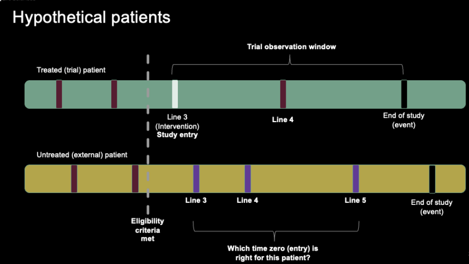
Two individual patients, one from the external dataset of interest and one from the trial of interest. Vertical lines represent the number of lines of therapy for a patient.
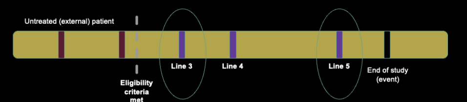
A single hypothetical patient from an external dataset of interest, demonstrating the multiple points that the patient could be considered to “start” the study.
Focusing in on this hypothetical patient, let us consider some conceptual start date. Note that the examples below are not intended to be genuine solutions to the issue at hand, rather, they are intended to provide an overview of how biases can be incorporated into analyses with study entry challenges.
If study entry (time zero) started at treatment line 3, this would represent the longest follow-up, and most favorable event-free duration for this patient. This will also be a source of bias, as we know the patient receives therapy up to line 5 and beyond.
Conversely, initiating time zero at the start of treatment line 5 would represent the shortest follow-up, and least favorable event-free duration. Again, this will be biased, as additional lines of therapy are typically associated with shorter event-free duration, and the shortened observational window may limit observations of safety events or longer-term outcomes.
Investigators may instead consider more directed approaches for setting time zero. For example, let us imagine that the median number of lines in the trial population is 4. We could therefore choose the line closest to the target for included patients, but in doing so effectively promote the biases identified above, as well as artificially reduce heterogeneity. Finally, an entirely random or pseudo-random start date could be chosen.
We focus above to describe a single patient for illustration purposes, but in a real study of this nature, these eligibility criteria apply across the entire population, and the impact can be highly variable depending on the patients included within the study.
These issues are not small scale or simply academic in nature, as highlighted by FDA Commissioner, Robert Califf, who recently noted that the “time-zero problem” is a major source of concern when reviewing applications incorporating evidence sensitive to misspecification of this phenomena. Striking the right balance is paramount to ensuring meaningful results and preventing skewed conclusions.
Case Study: Diabetic Retinopathy in Japan
To illustrate these challenges vividly, we delve into a recent publication featuring a unique set of characteristics conducted by Wakabayashi et al. 2022. The authors wanted to understand the impact of six different time zero strategies on estimating the impact of diabetic retinopathy (outcome) for patients using lipid-lowering agents (treated) and those who did not (non-use group). This study utilizes patient-level data from a substantial administrative claims dataset in Japan. Additionally, a diverse range of methods is employed, each exerting a significant influence on the observed differences between groups.
This study is unique for several reasons. First, the use of actual patient data to evaluate time-zero strategies is not commonplace, with many existing studies relying on simulated data to evaluate differences in strategies. Second, while many studies have historically highlighted time-zero choices for oncology applications for external control arms, this study presents an overview of a non-user comparative effectiveness design. Finally, the authors provided many subtle variations in the choice of time-zero strategy, helping to isolate several potentially influential bias propagation sources. The figure below shows the variety of approaches illustrated by the authors.
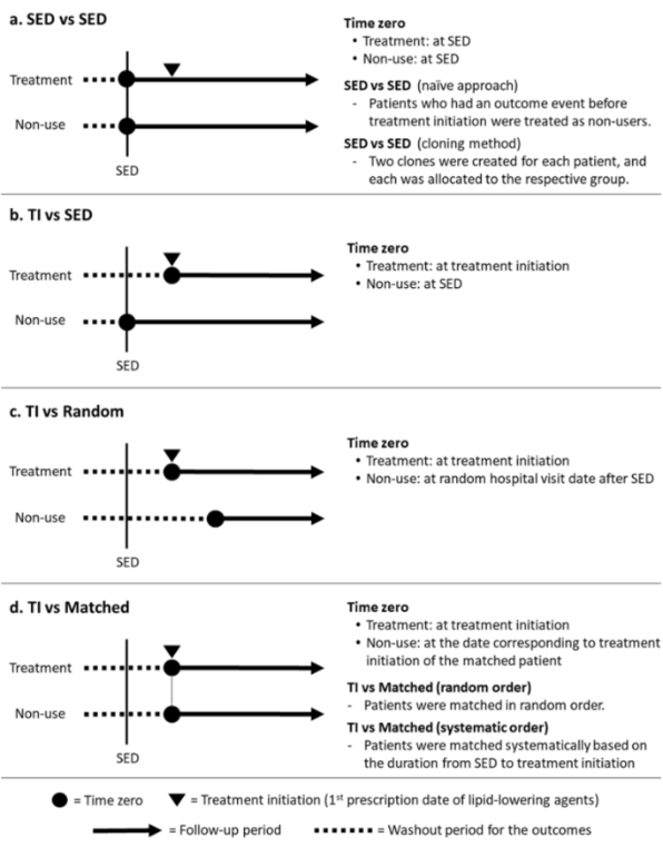
Acronyms: SED = Study Entry Data; TI = Treatment Initiation.
The authors provide a few scenarios covering topics likely familiar to readers. These include considering time zero at the first point of study (data) entry, or the first point of treatment among the population who were treated. They also highlight two more involved pre-processing approaches which have been suggested to help in bias mitigation.
Cloning Overview
One popular approach to navigate the intricacies of absolute and relative risk on survival outcomes is the “Cloning, censoring, and weighting” strategy. This involves assigning patients to all potential treatment strategies available within the observation window. Subsequently, patients are censored when their data no longer supports their treatment strategy. Given that cloning, if not accounted for, can introduce bias, inverse probability weighting is applied. This ensures that uncensored individuals receive a weight equivalent to the inverse probability of being uncensored. As such, patients with multiple possible study entry points are handled in a systematic manner reflecting the wide range of possible time-zero choices, whereas patients with more limited options are still retained.

Time Matching
Another compelling approach, as exemplified in this study, is matching the time-zero between treated and untreated patients. For treated patients, time-zero is marked by the initiation of treatment. Conversely, untreated patients are matched 1:1 to treated patients, aligning their study-entry date with that of their treated counterparts. This method often incorporates propensity scores to refine the matching process. Selecting suitable matches can be intricate, especially when multiple patients could potentially serve as appropriate matches. In this study, two approaches were adopted: “Random order” and “Systematic order”, each offering its own set of insights.
Results
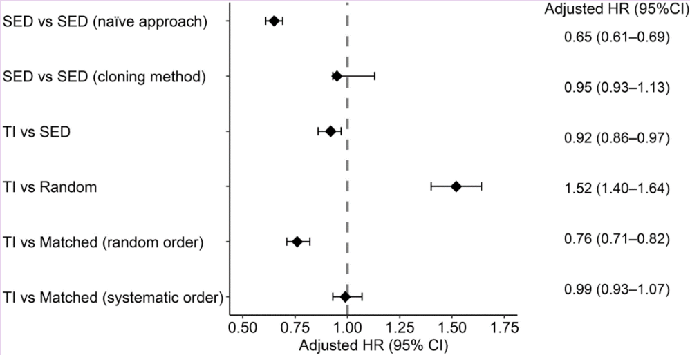
Under the naïve approach (where time-zero equals study entry date), the hazard ratio strongly favored the treated group (HR = 0.65). This finding underwent a complete reversal when comparing treatment initiation versus study entry date (HR = 1.52). Additionally, two approaches yielded non-significant findings. Even within the matching approaches, the choice between random or systematic order produced substantial variations in the identified hazard ratio.
Interpretation
As anticipated, specific approaches, such as the naïve one, tend to overestimate treatment effects. Notably, the reversal of results from the treatment initiation versus matching (random order) approach sparks intrigue. Matching is proposed as a means to minimize bias, and in the case of this study, the flipped signal could be attributed to patients removed from the non-use group due to events before time-zero, resulting in a longer period from study entry to time-zero. Indeed, the authors note that there was a longer period of study entry to time zero in the non-use group (306.6 days) when compared to the treatment group (154.4 days).
Limitations and Additional Considerations
While the issues of multiple eligibility pertain to a subset of data in observational research, it’s worth noting that not all study designs or research questions incorporate these complexities. For example, consider a study where the author is interested in what happens after the first lab test performed for all included patients. Various analytical strategies have been proposed, but many are tailored to specific use cases or simulation-based scenarios. Presently, no one strategy reigns supreme in terms of minimizing bias. Furthermore, in some applications, the absence of a clear “ground truth” complicates the determination of the “correct” answer. Finally, when considering the results of the current study, it’s important to note that the authors focused on exploring time-zero effects, without accounting for time-varying confounding or confounding by indication. These issues may influence the impact and interact with the differences in outputs from time-zero strategy choice.
Conclusion
Epidemiological research grapples with intricate designs where patients may possess multiple periods of eligibility. This extends beyond immortal time bias and requires meticulous consideration. While no single approach is universally applicable, one thing remains clear: naïve approaches consistently demonstrate a tendency to overestimate treatment effects. This is especially evident even when other “confounding-reducing” methods, such as propensity scores, are employed in isolation.